The standard map

The standard map

\[f(x,y) = (x+y+a\sin(x),y+a\sin(x))\]

is an area-preserving map on the 2-torus $[0,2\pi]^2$ resulting from a symplectic time-discretization of the planar pendulum. For $a = 0.971635$, its phase space shows the characteristic mixture of regular (periodic or quasi-periodic) and chaotic motion. Here, we repeat the experiment in Froyland & Junge (2015) and compute coherent structures.

We first visualize the phase space by plotting 500 iterates of 50 random seed points.

using Random

const a = 0.971635
f(x) = (rem2pi(x[1] + x[2] + a*sin(x[1]), RoundDown),
          rem2pi(x[2] + a*sin(x[1]), RoundDown))

X = Tuple{Float64,Float64}[]
for i in 1:50
    global X
    Random.seed!(i)
    x = 2π .* (rand(), rand())
    for i in 1:500
        x = f(x)
        push!(X,x)
    end
end

using Plots
gr(aspect_ratio=1, legend=:none)
fig = scatter(X, markersize=1)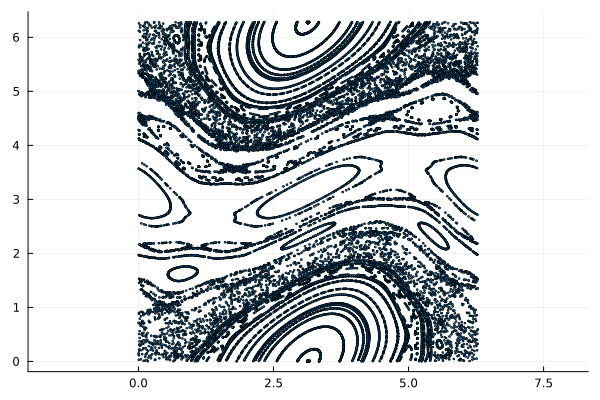

Approximating the Dynamic Laplacian by FEM methods is straightforward:

using CoherentStructures, Distances, Tensors

Df(x) = Tensor{2,2}((1.0+a*cos(x[1]), a*cos(x[1]), 1.0, 1.0))

n, ll, ur = 100, (0.0, 0.0), (2π, 2π)       # grid size, domain corners
ctx, _ = regularTriangularGrid((n, n), ll, ur)
pred = (x,y) -> peuclidean(x, y, [2π, 2π]) < 1e-9
bd = BoundaryData(ctx, pred)                # periodic boundary

I = one(Tensor{2,2})                        # identity matrix
Df2(x) = Df(f(x))⋅Df(x)                     # consider 2. iterate
cg(x) = 0.5*(I + dott(inv(Df2(x))))         # avg. inv. Cauchy-Green tensor

K = assembleStiffnessMatrix(ctx, cg, bdata=bd)
M = assembleMassMatrix(ctx, bdata=bd)
λ, v = CoherentStructures.get_smallest_eigenpairs(K, M, 6)

using Printf
title = [ @sprintf("\\lambda = %.3f", λ[i]) for i = 1:4 ]
p = [ plot_u(ctx, v[:,i], bdata=bd, title=title[i],
             clim=(-0.25, 0.25), cb=false) for i in 1:4 ]
fig = plot(p...)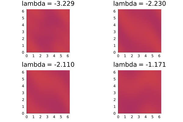

This page was generated using Literate.jl.