Working with trajectories

In the following, we demonstrate how to use coherent structure detection methods that work directly on trajectory data sets. These include the graph Laplace-based and the transfer operator-based methods for approximating the dynamic Laplacian. For simplicity, we will demonstrate the methods based on trajectories obtained from integrating the Bickley jet velocity field.

Graph Laplace-based methods

In the following, we demonstrate how to apply several graph Laplace-based coherent structure detection methods. For references and technical details, we refer to the corresponding Graph Laplacian/diffusion maps-based LCS methods page.

As an example, this is how we can add more processes to run code in parallel.

using Distributed
(nprocs() == 1) && addprocs()

We first load our package, some dependencies, and define the vector field.

@everywhere using CoherentStructures, StreamMacros
using Distances, Plots
const bickleyJet = @velo_from_stream psi begin
    psi  = psi₀ + psi₁
    psi₀ = - U₀ * L₀ * tanh(y / L₀)
    psi₁ =   U₀ * L₀ * sech(y / L₀)^2 * re_sum_term

    re_sum_term = Σ₁ + Σ₂ + Σ₃

    Σ₁ = ε₁ * cos(k₁*(x - c₁*t))
    Σ₂ = ε₂ * cos(k₂*(x - c₂*t))
    Σ₃ = ε₃ * cos(k₃*(x - c₃*t))

    k₁ = 2/r₀    ; k₂ = 4/r₀   ; k₃ = 6/r₀
    ε₁ = 0.0075  ; ε₂ = 0.15   ; ε₃ = 0.3
    c₂ = 0.205U₀ ; c₃ = 0.461U₀; c₁ = c₃ + (√5-1)*(c₂-c₃)
    U₀ = 62.66e-6; L₀ = 1770e-3; r₀ = 6371e-3
end

Next, we define the usual flow parameters. For visualization convenience, we use a regular grid at initial time.

const tspan = range(10*24*3600.0, stop=30*24*3600.0, length=41)
m = 120; n = 41; N = m*n
x = range(0.0, stop=20.0, length=m)
y = range(-3.0, stop=3.0, length=n)
f = u -> flow(bickleyJet, u, tspan, tolerance=1e-4)
particles = vec(tuple.(x, y'))
trajectories = pmap(f, particles; batch_size=ceil(Int, N/nprocs()^2))

The flow is defined on a cylinder with the following periods in x and y. The variable metric defines the (spatial) distance metric.

periods = [6.371π, Inf]
metric = PeriodicEuclidean(periods)

We would like calculate 6 diffusion coordinates for each example.

n_coords = 6

We now illustrate some of the different graph Laplace-based methods, and simply visualize some eigenvectors, mostly without further postprocessing.

Spectral-clustering approach/L_1 time averaging [Hadjighasem, Karrasch, Teramoto & Haller, 2016]

ε = 1.0
kernel = gaussian(ε)
P = sparse_diff_op(trajectories, Neighborhood(gaussiancutoff(ε/20)), kernel; metric=STmetric(metric, 1))
λ, Ψ = diffusion_coordinates(P, n_coords)

We plot the second and third eigenvectors.

field = permutedims(reshape(Ψ[:, 2], m, n))
fig = Plots.heatmap(x, y, field, aspect_ratio=1, color=:viridis)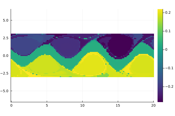

field = permutedims(reshape(Ψ[:, 3], m, n))
fig = Plots.heatmap(x, y, field, aspect_ratio=1, color=:viridis)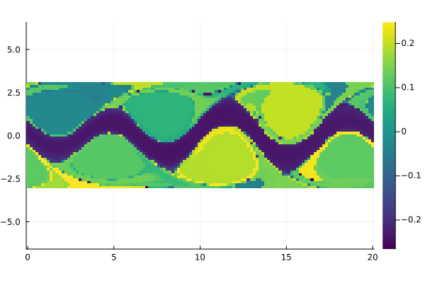

Another sparsification option is k-nearest neighbors. The following is a demonstration for 400 nearest, non-mutual neighbors. For the mutual nearest neighbors sparsification, choose MutualKNN().

P = sparse_diff_op(trajectories, KNN(200), gaussian(10); metric=STmetric(metric, Inf))
λ, Ψ = diffusion_coordinates(P, n_coords)

field = permutedims(reshape(Ψ[:, 2], m, n))
fig = Plots.heatmap(x, y, field, aspect_ratio=1, color=:viridis)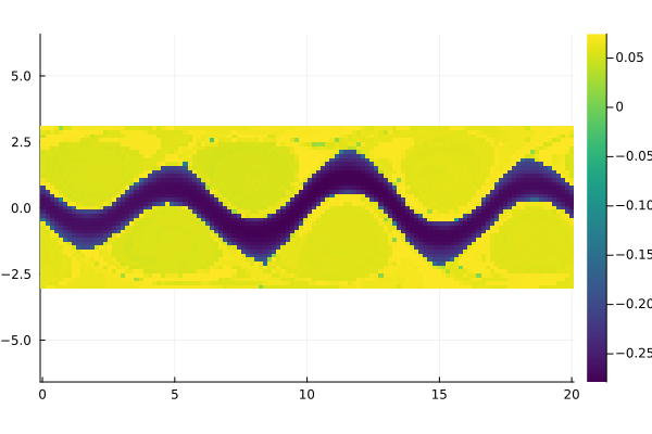

field = permutedims(reshape(Ψ[:, 3], m, n))
fig = Plots.heatmap(x, y, field, aspect_ratio=1, color=:viridis)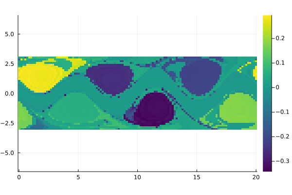

Use of SEBA to extract features

For feature extraction from operator eigenvectors, one may use the "SEBA" method developed by [Froyland, Rock & Sakellariou, 2019].

Ψ2 = SEBA(Ψ)

We plot two of the SEBA features extracted.

field = permutedims(reshape(Ψ2[:, 1], m, n))
fig = Plots.heatmap(x, y, field, aspect_ratio=1, color=:viridis)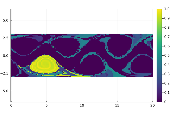

field = permutedims(reshape(Ψ2[:, 2], m, n))
fig = Plots.heatmap(x, y, field, aspect_ratio=1, color=:viridis)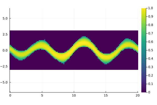

Space-time diffusion maps [Banisch & Koltai, 2017]

import Statistics: mean
σ = 1e-3
kernel = gaussian(σ)
P = sparse_diff_op_family(trajectories, Neighborhood(gaussiancutoff(σ)), kernel, mean; metric=metric)
λ, Ψ = diffusion_coordinates(P, n_coords)

field = permutedims(reshape(Ψ[:, 2], m, n))
fig = Plots.heatmap(x, y, field, aspect_ratio=1, color=:viridis)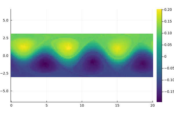

field = permutedims(reshape(Ψ[:, 3], m, n))
fig = Plots.heatmap(x, y, field, aspect_ratio=1, color=:viridis)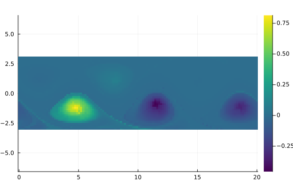

Network-based approach [Padberg-Gehle & Schneide, 2017]

ε = 0.2
P = sparse_diff_op_family(trajectories, Neighborhood(ε), Base.one, row_normalize!∘unionadjacency;
                            α=0, metric=metric)
λ, Ψ = diffusion_coordinates(P, n_coords)

field = permutedims(reshape(Ψ[:, 2], m, n))
fig = Plots.heatmap(x, y, field, aspect_ratio=1, color=:viridis)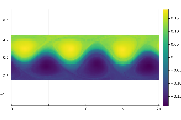

field = permutedims(reshape(Ψ[:, 3], m, n))
fig = Plots.heatmap(x, y, field, aspect_ratio=1, color=:viridis)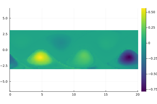

Time coupled diffusion coordinates [Marshall & Hirn, 2018]

σ = 1e-3
kernel = gaussian(σ)
P = sparse_diff_op_family(trajectories, Neighborhood(gaussiancutoff(σ)), kernel; metric=metric)
λ, Ψ = diffusion_coordinates(P, n_coords)

field = permutedims(reshape(Ψ[:, 2], m, n))
fig = Plots.heatmap(x, y, field, aspect_ratio=1, color=:viridis)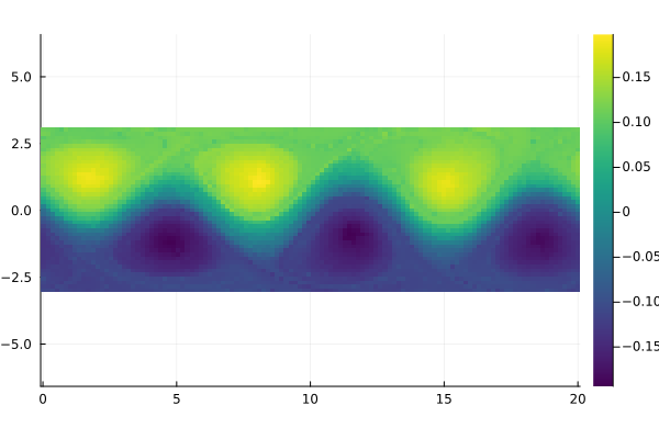

field = permutedims(reshape(Ψ[:, 3], m, n))
fig = Plots.heatmap(x, y, field, aspect_ratio=1, color=:viridis)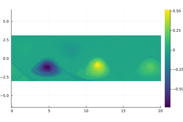

FEM adaptive TO method

We first generate some trajectories on a set of n random points for the rotating double gyre flow.

using StreamMacros, CoherentStructures, Random, Plots, Clustering
const rot_double_gyre = @velo_from_stream Ψ_rot_dgyre begin
    st          = heaviside(t)*heaviside(1-t)*t^2*(3-2*t) + heaviside(t-1)
    heaviside(x)= 0.5*(sign(x) + 1)
    Ψ_P         = sin(2π*x)*sin(π*y)
    Ψ_F         = sin(π*x)*sin(2π*y)
    Ψ_rot_dgyre = (1-st) * Ψ_P + st * Ψ_F
end

n = 500
ts = range(0, stop=1.0, length=20)
Random.seed!(1234)
xs, ys = rand(n), rand(n)
particles = zip(xs, ys)
trajectories = [flow(rot_double_gyre, p, ts) for p in particles]

Based on the initial particle positions we generate a triangulation. If this call fails or does not return, the initial positions may not be unique. In that case, simply generate a different set of random initial positions.

ctx, _ = irregularDelaunayGrid(particles)

Next, we generate the stiffness and mass matrices and solve the generalized eigenproblem.

S = adaptiveTOCollocationStiffnessMatrix(ctx, (i, ts) -> trajectories[i], ts; flow_map_mode=1)
M = assembleMassMatrix(ctx)
λ, V = CoherentStructures.get_smallest_eigenpairs(S, M, 6)

We can plot the computed spectrum.

fig = plot_real_spectrum(λ, label="")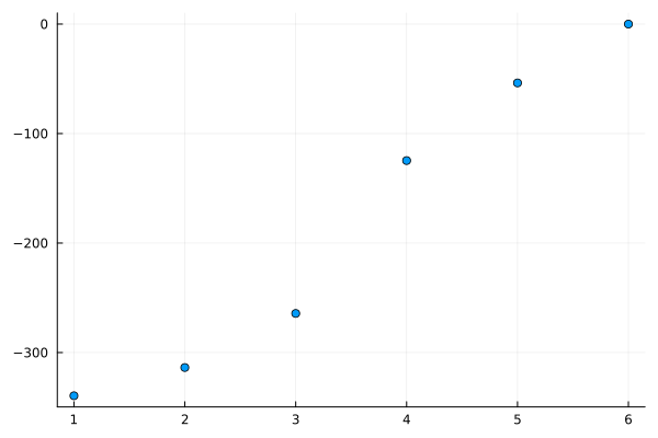

We may extract coherent vortices with k-means clustering.

function iterated_kmeans(iterations, args...)
    best = kmeans(args...)
    for i in 1:(iterations - 1)
        cur = kmeans(args...)
        if cur.totalcost < best.totalcost
            best = cur
        end
    end
    return best.assignments
end

partitions = 3
clusters = iterated_kmeans(20, permutedims(V[:, 2:partitions]), partitions)

A simple scatter plot visualization looks as follows.

fig = scatter(xs, ys, zcolor=clusters[ctx.node_to_dof], markersize=8, labels="")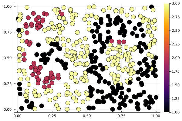

Alternatively, we may also plot the cluster assignments on the whole irregular grid.

fig = plot_u(ctx, float(clusters), 400, 400;
                color=:viridis,
                colorbar=:none,
                title="$partitions-partition of rotating double gyre")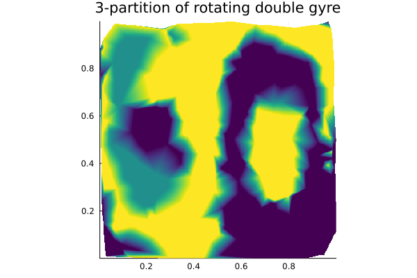

This page was generated using Literate.jl.