Bickley jet

The Bickley jet flow is a kinematic idealized model of a meandering zonal jet flanked above and below by counterrotating vortices. It was introduced by Rypina et al.; cf. also del‐Castillo‐Negrete and Morrison.

The Bickley jet is described by a time-dependent velocity field arising from a stream-function. The corresponding velocity field can be conveniently defined using the @velo_from_stream macro from StreamMacros.jl:

using Distributed
nprocs() == 1 && addprocs()

@everywhere using CoherentStructures, StreamMacros
const bickley = @velo_from_stream psi begin
    psi  = psi₀ + psi₁
    psi₀ = - U₀ * L₀ * tanh(y / L₀)
    psi₁ =   U₀ * L₀ * sech(y / L₀)^2 * re_sum_term

    re_sum_term = Σ₁ + Σ₂ + Σ₃

    Σ₁ = ε₁ * cos(k₁*(x - c₁*t))
    Σ₂ = ε₂ * cos(k₂*(x - c₂*t))
    Σ₃ = ε₃ * cos(k₃*(x - c₃*t))

    k₁ = 2/r₀    ; k₂ = 4/r₀   ; k₃ = 6/r₀
    ε₁ = 0.0075  ; ε₂ = 0.15   ; ε₃ = 0.3
    c₂ = 0.205U₀ ; c₃ = 0.461U₀; c₁ = c₃ + (√5-1)*(c₂-c₃)
    U₀ = 62.66e-6; L₀ = 1770e-3; r₀ = 6371e-3
end

Now, bickley is a callable function with the standard OrdinaryDiffEq signature (u, p, t) with state u, (unused) parameter p and time t.

Geodesic vortices

Here we briefly demonstrate how to find material barriers to diffusive transport; see Geodesic elliptic material vortices for references and details.

@everywhere using OrdinaryDiffEq, Tensors
q = 81
const tspan = range(0., stop=3456000., length=q)
ny = 61
nx = (22ny) ÷ 6
xmin, xmax, ymin, ymax = 0.0 - 2.0, 6.371π + 2.0, -3.0, 3.0
xspan = range(xmin, stop=xmax, length=nx)
yspan = range(ymin, stop=ymax, length=ny)
P = tuple.(xspan, yspan')
const δ = 1.e-6
const D = SymmetricTensor{2,2}((2., 0., 1/2))
mCG_tensor = u -> av_weighted_CG_tensor(bickley, u, tspan, δ; D=(_ -> D), tolerance=1e-6, solver=Tsit5())

C̅ = pmap(mCG_tensor, P; batch_size=ceil(Int, length(P)/nprocs()^2))
p = LCSParameters(2.0)
vortices, singularities = ellipticLCS(C̅, xspan, yspan, p)

The result is visualized as follows:

using Plots
trace = tensor_invariants(C̅)[5]
fig = plot_vortices(vortices, singularities, (xmin, ymin), (xmax, ymax);
    bg=trace, xspan=xspan, yspan=yspan, title="DBS field and transport barriers", showlabel=true)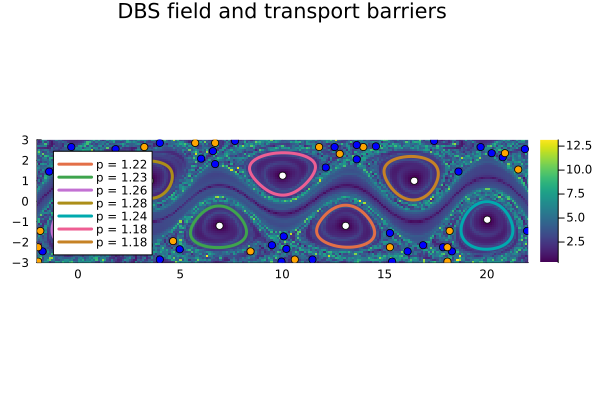

FEM-based Methods

Assume we have setup the bickley function using the @velo_from_stream macro as described above. We are working on a periodic domain in one direction:

using Distances
LL = (0.0, -3.0); UR = (6.371π, 3.0)
ctx, _ = regularP2TriangularGrid((50, 15), LL, UR, quadrature_order=2)
predicate = (p1, p2) -> peuclidean(p1, p2, [6.371π, Inf]) < 1e-10
bdata = BoundaryData(ctx, predicate, []);

Using a FEM-based method to compute coherent structures:

cgfun = x -> mean_diff_tensor(bickley, x, range(0.0, stop=40*3600*24, length=81), 1.e-8; tolerance=1e-5)

K = assembleStiffnessMatrix(ctx, cgfun, bdata=bdata)
M = assembleMassMatrix(ctx, bdata=bdata)
λ, v = CoherentStructures.get_smallest_eigenpairs(K, M, 10)

import Plots
fig_spectrum = plot_real_spectrum(λ)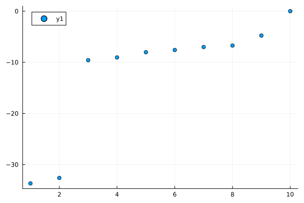

K-means clustering yields the coherent vortices.

using Clustering
ctx2, _ = regularTriangularGrid((200, 60), LL, UR)
v_upsampled = sample_to(v, ctx, ctx2, bdata=bdata)

function iterated_kmeans(numiterations, args...)
    best = kmeans(args...)
    for i in 1:(numiterations - 1)
        cur = kmeans(args...)
        if cur.totalcost < best.totalcost
            best = cur
        end
    end
    return best
end

n_partition = 8
res = iterated_kmeans(20, permutedims(v_upsampled[:,2:n_partition]), n_partition)
u = kmeansresult2LCS(res)
u_combined = sum([u[:,i] * i for i in 1:n_partition])
fig = plot_u(ctx2, u_combined, 400, 400;
    color=:rainbow, colorbar=:none, title="$n_partition-partition of Bickley jet")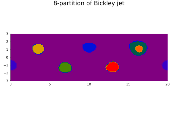

This page was generated using Literate.jl.