Geostrophic ocean flow
This example is also available as a Jupyter notebook: ocean_flow.ipynb, and as an executable julia file ocean_flow.jl.
For a more realistic application, we consider an unsteady ocean surface velocity data set obtained from satellite altimetry measurements produced by SSALTO/DUACS and distributed by AVISO. The particular space-time window has been used several times in the literature.
Below is a video showing advection of the initial 90-day DBS field for 90 days.
Geodesic vortices
Here, we demonstrate how to detect material barriers to diffusive transport.
using Distributed
nprocs() == 1 && addprocs()

@everywhere using CoherentStructures, OrdinaryDiffEq
Next, we load and interpolate the velocity data sets.
using JLD2
xs, ys, ts, us, vs = load("docs/examples/Ocean_geostrophic_velocity.jld2", "Lon", "Lat", "Time", "UT", "VT")
const uv = interpolateVF(xs, ys, ts, us, vs)
Now, we set up the computational problem.
q = 91
t_initial = minimum(ts)
t_final = t_initial + 90
const tspan = range(t_initial, stop=t_final, length=q)
xmin, xmax, ymin, ymax = -4.0, 7.5, -37.0, -28.0
nx = 300
ny = floor(Int, (ymax - ymin) / (xmax - xmin) * nx)
xspan = range(xmin, stop=xmax, length=nx)
yspan = range(ymin, stop=ymax, length=ny)
P = tuple.(xspan, permutedims(yspan))
const δ = 1.e-5
mCG_tensor = u -> av_weighted_CG_tensor(interp_rhs, u, tspan, δ;
    p=uv, tolerance=1e-6, solver=Tsit5())
Next, we compute the averaged weighted Cauchy-Green tensor field and extract elliptic LCSs.
C̅ = pmap(mCG_tensor, P; batch_size=ceil(Int, length(P)/nprocs()^2))
p = LCSParameters(2.5)
vortices, singularities = ellipticLCS(C̅, xspan, yspan, p)
Let us compute the area of each vortex has and whether it rotates in a clockwise fashion.
area.(vortices), clockwise.(vortices, interp_rhs, t_initial, p=uv)Finally, the result is visualized as follows.
using Plots
trace = tensor_invariants(C̅)[5]
fig = plot_vortices(vortices, singularities, (xmin, ymin), (xmax, ymax);
    bg=trace, xspan=xspan, yspan=yspan, title="DBS field and transport barriers", showlabel=true)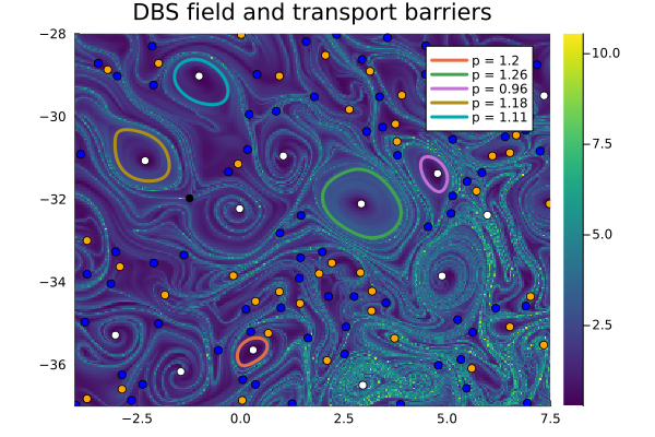
Objective Eulerian coherent structures (OECS)
With only minor modifications, we are also able to compute OECSs. We start by loading some packages and define the rate-of-strain tensor function.
using Interpolations, Tensors, StaticArrays

const V = scale(interpolate(SVector{2}.(us[:,:,1], vs[:,:,1]), BSpline(Quadratic(Free(OnGrid())))), xs, ys)

rate_of_strain_tensor(xin) = let V=V
    x, y = xin
    grad = Interpolations.gradient(V, x, y)
    symmetric(Tensor{2,2}((grad[1][1], grad[1][2], grad[2][1], grad[2][2])))
end
To make life more exciting, we choose a larger domain.
xmin, xmax, ymin, ymax = -12.0, 7.0, -38.1, -22.0
nx = 950
ny = floor(Int, (ymax - ymin) / (xmax - xmin) * nx)
xspan = range(xmin, stop=xmax, length=nx)
yspan = range(ymin, stop=ymax, length=ny)
P = tuple.(xspan, permutedims(yspan))
Next, we evaluate the rate-of-strain tensor on the grid and compute OECSs. As there tend to be many 3 wedge + trisector-type singularity combinations with OECSs, we enable the combine_31 heuristic.
S = rate_of_strain_tensor.(P)
p = LCSParameters(boxradius=2.5, pmin=-1, pmax=1, merge_heuristics=[Combine20(), Combine31()])
vortices, singularities = ellipticLCS(S, xspan, yspan, p; outermost=true)
Finally, the result is visualized as follows, white are elliptic singularities, blue are trisectors and orange are wedges
λ₁ = tensor_invariants(S)[1]
fig = plot_vortices(vortices, singularities, (xmin, ymin), (xmax, ymax);
    bg=λ₁, xspan=xspan, yspan=yspan, logBg=false, title="Minor rate-of-strain field and OECSs")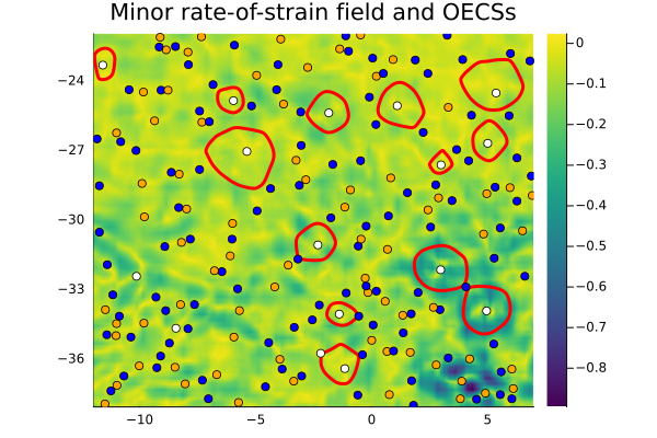
FEM-based methods
Here we showcase how the adaptive TO method can be used to calculate coherent sets.
First we setup the problem.
using CoherentStructures
import JLD2, OrdinaryDiffEq, Plots

xs, ys, ts, us, vs = load("Ocean_geostrophic_velocity.jld2", "Lon", "Lat", "Time", "UT", "VT")

const UV = interpolateVF(xs, ys, ts, us, vs)
Next, we define a flow function from it.
t_initial = minimum(ts)
t_final = t_initial + 90
const times = [t_initial, t_final]
flow_map(u0) = flow(interp_rhs, u0, times; p=UV, tolerance=1e-5, solver=OrdinaryDiffEq.BS5())[end]
Next, we set up the domain. We want to use zero Dirichlet boundary conditions here.
LL = (-4.0, -34.0)
UR = (6.0, -28.0)
ctx, _  = regularTriangularGrid((150, 90), LL, UR)
bdata = getHomDBCS(ctx, "all");
For the TO method, we seek generalized eigenpairs involving the bilinear form
\[a_h(u,v) = \frac{1}{2} \left(a_0(u,v) + a_1(I_h u, I_h v) \right).\]
Here, $a_0$ is the weak form of the Laplacian on the initial domain, and $a_1$ is the weak form of the Laplacian on the final domain. The operator $I_h$ is an interpolation operator onto the space of test functions on the final domain.
For the adaptive TO method, we use pointwise nodal interpolation (i.e. collocation) and the mesh on the final domain is obtained by doing a Delaunay triangulation on the images of the nodal points of the initial domain. This results in the representation matrix of $I_h$ being the identity, so in matrix form we get:
\[S = 0.5(S_0 + S_1)\]
where $S_0$ is the stiffness matrix for the triangulation at initial time, and $S_1$ is the stiffness matrix for the triangulation at final time.
M = assembleMassMatrix(ctx, bdata=bdata)
S0 = assembleStiffnessMatrix(ctx)
S1 = adaptiveTOCollocationStiffnessMatrix(ctx, flow_map)
Averaging matrices and applying boundary conditions yields
S = applyBCS(ctx, 0.5(S0 + S1), bdata);We can now solve the eigenproblem.
λ, v = CoherentStructures.get_smallest_eigenpairs(S, M, 6);We upsample the eigenfunctions and then cluster.
using Clustering

ctx2, _ = regularTriangularGrid((200, 120), LL, UR)
v_upsampled = sample_to(v, ctx, ctx2, bdata=bdata)

function iterated_kmeans(numiterations, args...)
    best = kmeans(args...)
    for i in 1:(numiterations - 1)
        cur = kmeans(args...)
        if cur.totalcost < best.totalcost
            best = cur
        end
    end
    return best
end

n_partition = 4
res = iterated_kmeans(20, permutedims(v_upsampled[:,1:(n_partition-1)]), n_partition)
u = kmeansresult2LCS(res)
u_combined = sum([u[:,i] * i for i in 1:n_partition])
fig = plot_u(ctx2, u_combined, 200, 200;
    color=:viridis, colorbar=:none, title="$n_partition-partition of Ocean Flow")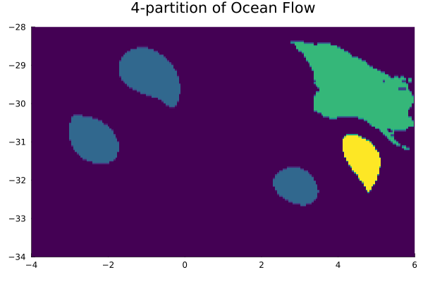
This page was generated using Literate.jl.