Rotating double gyre
This example is also available as a Jupyter notebook: rot_double_gyre.ipynb, and as an executable julia file rot_double_gyre.jl.
Description
The rotating double gyre model was introduced by Mosovsky & Meiss. It can be derived from the stream function
\[\psi(x,y,t)=(1−s(t))\psi_P +s(t)\psi_F \\ \psi_P (x, y) = \sin(2\pi x) \sin(\pi y) \\ \psi_F (x, y) = \sin(\pi x) \sin(2\pi y)\]
where $s$ is (usually taken to be) a cubic interpolating function satisfying $s(0) = 0$ and $s(1) = 1$. It therefore interpolates two double-gyre-type velocity fields, from horizontally to vertically arranged counter-rotating gyres. The corresponding velocity field can be conveniently defined using the @velo_from_stream macro from StreamMacros.jl:
using Distributed
nprocs() == 1 && addprocs()

@everywhere using StreamMacros
const rot_double_gyre = @velo_from_stream Ψ_rot_dgyre begin
    st          = heaviside(t)*heaviside(1-t)*t^2*(3-2*t) + heaviside(t-1)
    heaviside(x)= 0.5*(sign(x) + 1)
    Ψ_P         = sin(2π*x)*sin(π*y)
    Ψ_F         = sin(π*x)*sin(2π*y)
    Ψ_rot_dgyre = (1-st) * Ψ_P + st * Ψ_F
end
FEM-Based Methods
The following code demonstrates how to use these methods.
using CoherentStructures
LL, UR = (0.0, 0.0), (1.0, 1.0)
ctx, _ = regularTriangularGrid((50, 50), LL, UR)

A = x -> mean_diff_tensor(rot_double_gyre, x, [0.0, 1.0], 1.e-10, tolerance= 1.e-4)
K = assembleStiffnessMatrix(ctx, A)
M = assembleMassMatrix(ctx)
λ, v = CoherentStructures.get_smallest_eigenpairs(-K, M, 6);
This velocity field is given by the rot_double_gyre function. The third argument to mean_diff_tensor is a vector of time instances at which we evaluate (and subsequently average) the pullback diffusion tensors. The fourth parameter is the step size δ used for the finite-difference scheme, tolerance is passed to the ODE solver from DifferentialEquations.jl. In the above, A(x) approximates the mean diffusion tensor given by
\[A(x) = \sum_{t \in \mathcal T}(D\Phi^t(x))^{-1} (D\Phi^t x)^{-T}\]
The eigenfunctions saved in v approximate those of $\Delta^{dyn}$
import Plots
res = [plot_u(ctx, v[:,i], 100, 100, colorbar=:none, clim=(-3,3)) for i in 1:6];
fig = Plots.plot(res..., margin=-10Plots.px)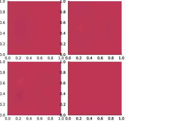
Looking at the spectrum, there appears a gap after the third eigenvalue.
spectrum_fig = Plots.scatter(1:6, real.(λ))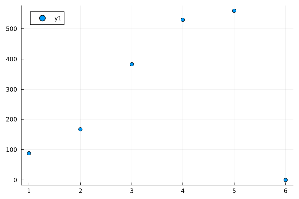
We can use the Clustering.jl package to compute coherent structures from the first two nontrivial eigenfunctions:
using Clustering

ctx2, _ = regularTriangularGrid((200, 200))
v_upsampled = sample_to(v, ctx, ctx2)

numclusters=2
res = kmeans(permutedims(v_upsampled[:,2:numclusters+1]), numclusters + 1)
u = kmeansresult2LCS(res)
res = Plots.plot([plot_u(ctx2, u[:,i], 200, 200, c=:viridis, cbar=:none) for i in 1:3]...)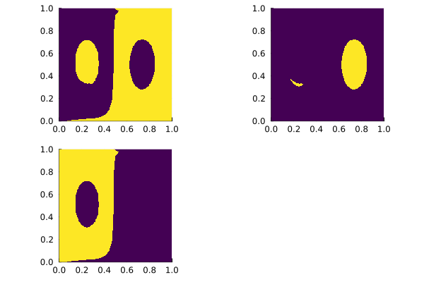
Geodesic vortices
Here, we demonstrate how to calculate black-hole vortices, see Geodesic elliptic material vortices for references and details.
@everywhere using CoherentStructures, OrdinaryDiffEq
q = 21
const tspan = range(0., stop=1., length=q)
nx = ny = 101
xmin, xmax, ymin, ymax = 0.0, 1.0, 0.0, 1.0
xspan = range(xmin, stop=xmax, length=nx)
yspan = range(ymin, stop=ymax, length=ny)
P = tuple.(xspan, permutedims(yspan))
const δ = 1.e-6
mcg_tensor = u -> av_weighted_CG_tensor(rot_double_gyre, u, tspan, δ; tolerance=1e-6, solver=Tsit5())

C̅ = pmap(mcg_tensor, P; batch_size=ceil(Int, length(P)/nprocs()^2))
p = LCSParameters(0.5)
vortices, singularities = ellipticLCS(C̅, xspan, yspan, p; outermost=true)
The results are then visualized as follows.
using Plots
trace = tensor_invariants(C̅)[5]
fig = plot_vortices(vortices, singularities, (xmin, ymin), (xmax, ymax);
    bg=trace, xspan=xspan, yspan=yspan, title="DBS field and transport barriers", showlabel=true, clims=(0,5))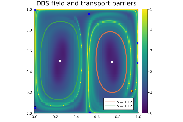
This page was generated using Literate.jl.