Material diffusion barriers in a turbulent flow
This example is also available as a Jupyter notebook: turbulence.ipynb, and as an executable julia file turbulence.jl.
The following script reproduces partially the two-dimensional turbulence simulation performed in the paper Fast and robust computation of coherent Lagrangian vortices on very large two-dimensional domains, jointly written by Daniel Karrasch and Nathanael Schilling, which appeared in SMAI Journal of Computational Mathematics.
As usual, we rely on several, open-source Julia packages. The following commands show how to install specific versions such that this script works out of the box. Users are encouraged, however, to test up-to-date versions, i.e., without pinning the specific versions. Installing (and pinning) these packages is required only the first time this script is run.
import Pkg
Pkg.add("FourierFlows")
Pkg.add("GeophysicalFlows")
Pkg.add("Plots")
Pkg.add(Pkg.PackageSpec(url="https://github.com/CoherentStructures/CoherentStructures.jl.git"))
Pkg.add(Pkg.PackageSpec(url="https://github.com/CoherentStructures/OceanTools.jl.git"))
Pkg.pin(Pkg.PackageSpec(name="FourierFlows", version="0.4.5"))
Pkg.pin(Pkg.PackageSpec(name="GeophysicalFlows", version="0.5.1"))
Generating a turbulent velocity field
We begin by loading required packages and by setting up a computational domain.
using FourierFlows, GeophysicalFlows, GeophysicalFlows.TwoDNavierStokes, Plots, Random
Random.seed!(1234)
mygrid = TwoDGrid(256, 2π)
x, y = gridpoints(mygrid)
xs = ys = range(-π, stop=π, length=257)[1:end-1];
To avoid decay of the flow we employ stochastic forcing. The code below is modified from an example given in the GeophysicalFlows.jl documentation.
ε = 0.001 # Energy injection rate
kf, dkf = 6, 2.0 # Waveband where to inject energy
Kr = [mygrid.kr[i] for i=1:mygrid.nkr, j=1:mygrid.nl]
force2k = @. exp(-(sqrt(mygrid.Krsq) - kf)^2 / (2 * dkf^2))
force2k[(mygrid.Krsq .< 2.0^2) .| (mygrid.Krsq .> 20.0^2) .| (Kr .< 1) ] .= 0
ε0 = FourierFlows.parsevalsum(force2k .* mygrid.invKrsq/2.0,
                                mygrid) / (mygrid.Lx*mygrid.Ly)
force2k .= ε/ε0 * force2k
function calcF!(Fh, sol, t, cl, args...)
    eta = exp.(2π * im * rand(Float64, size(sol))) / sqrt(cl.dt)
    eta[1,1] = 0
    @. Fh = eta * sqrt(force2k)
    nothing
end
We now setup the remaining parameters used in the simulation. We numerically solve the vorticity (transport) equation
\[\partial_t \zeta = - u\cdot \nabla \zeta -\nu\zeta + f.\]
Here $u(x,y) = (u_1(x,y),u_2(x,y))^T$ is the (incompressible) velocity field, and $\zeta = \partial_x u_2 - \partial_y u_1$ is its vorticity. The parameter $\nu$ has the value $10^{-2}$ and is the coefficient of the drag term, $f$ represents the forcing.
prob = TwoDNavierStokes.Problem(nx=256, Lx=2π, ν=1e-2, nν=0, dt=1e-2,
    stepper="FilteredRK4", calcF=calcF!, stochastic=true)
TwoDNavierStokes.set_zeta!(prob, GeophysicalFlows.peakedisotropicspectrum(mygrid, 2, 0.5))

#md

using Distributed
addprocs()
using SharedArrays
we use these variables to store the result
us = SharedArray{Float64}(256, 256, 400)
vs = SharedArray{Float64}(256, 256, 400)
zs = SharedArray{Float64}(256, 256, 400);
We run this simulation until $t=500$ to work in a statistically equilibrated state, and then save the result at time steps of size 0.2.
@time stepforward!(prob, round(Int, 500 / prob.clock.dt))
@time for i in 1:400
    stepforward!(prob, 20); TwoDTurb.updatevars!(prob)
    vs[:,:,i] = prob.vars.v
    us[:,:,i] = prob.vars.u
    zs[:,:,i] = prob.vars.zeta
end
The generation of the velocity field by the above code takes on the order of 10 minutes on a modern notebook. Below, we show the vorticity field at $t = 500$.
heatmap(xs, ys, zs[:,:,1];
    color=:viridis, aspect_ratio=1, xlim=extrema(xs), ylim=extrema(ys))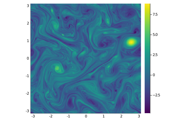
Material diffusion barrier detection
We first setup a periodic interpolation of the velocity field, using the OceanTools.jl package.
@everywhere using CoherentStructures, OceanTools
const CS = CoherentStructures
const OT = OceanTools
ts = range(0.0, step=20prob.clock.dt, length=400)
const uv = OT.ItpMetadata(xs, ys, ts, (us, vs), OT.periodic, OT.periodic, OT.flat);
We are now ready to compute material barriers.
vortices, singularities, bg = CS.materialbarriers(
       uv_trilinear, xs, ys, range(0.0, stop=5.0, length=11),
       LCSParameters(boxradius=π/2, indexradius=0.1, pmax=1.4,
                     merge_heuristics=[combine_20_aggressive]),
       p=uv, on_torus=true);
The materialbarriers function calculates the transport tensor field $\mathbf{T}$ used in the material-barriers approach (using finite differences for the linearized flow map $D\Phi$) and calculates material barriers. The result is shown below.
plot_vortices(vortices, singularities, [-π, -π], [π, π];
    bg=bg, xspan=xs, yspan=ys, include_singularities=true, barrier_width=4, barrier_color=:red,
    colorbar=:false, aspect_ratio=1)
We plot the detected vortices on top of the vorticity field.
plot_vortices(vortices, singularities, [-π, -π], [π, π];
    bg=zs[:,:,1], xspan=xs, yspan=ys, logBg=false, include_singularities=false, barrier_width=3, barrier_color=:red,
    colorbar=:false, aspect_ratio=1)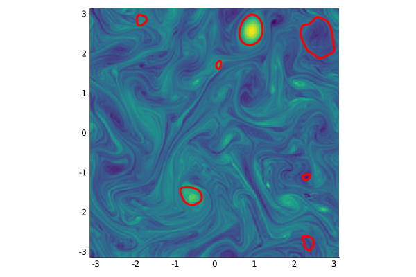
Next, we advect them forwards in time.
vortexflow = vortex -> flow(uv_trilinear, vortex, [0., 5.]; p=uv)[end]
plot_vortices(vortexflow.(vortices), singularities, [-π, -π], [π, π];
    bg=zs[:,:,26], xspan=xs, yspan=ys, logBg=false, include_singularities=false, barrier_width=3, barrier_color=:red,
    colorbar=:false, aspect_ratio=1)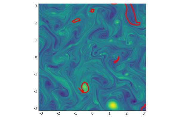
One of the vortices has been advected so that it is no longer in the field of view of the image, and the plotting function doesn't know that the domain is periodic.
This page was generated using Literate.jl.