Material diffusion barriers
This example is also available as a Jupyter notebook: diffbarriers.ipynb, and as an executable julia file diffbarriers.jl.
The following script reproduces partially the simulations performed in the paper Material barriers to diffusive and stochastic transport, jointly written by George Haller, Daniel Karrasch and Florian Kogelbauer, which appeared in PNAS.
Bickley-jet flow
The Bickley jet flow is a kinematic idealized model of a meandering zonal jet flanked above and below by counterrotating vortices. It was introduced by Rypina et al.; cf. also del‐Castillo‐Negrete and Morrison.
The Bickley jet is described by a time-dependent velocity field arising from a stream-function. The corresponding velocity field can be constructed by means of the StreamMacros.jl package.
import Pkg
Pkg.add(Pkg.PackageSpec(url="https://github.com/CoherentStructures/CoherentStructures.jl.git"))
Pkg.add(Pkg.PackageSpec(url="https://github.com/CoherentStructures/StreamMacros.jl"))
Pkg.add(["OrdinaryDiffEq", "Tensors", "JLD2", "Plots"])
Next, we turn on parallel computing, load the relevant packages on all available workers and define the velocity field.
using Distributed
nprocs() == 1 && addprocs()

@everywhere using StreamMacros
const bickley = @velo_from_stream psi begin
    psi  = psi₀ + psi₁
    psi₀ = - U₀ * L₀ * tanh(y / L₀)
    psi₁ =   U₀ * L₀ * sech(y / L₀)^2 * re_sum_term

    re_sum_term = Σ₁ + Σ₂ + Σ₃

    Σ₁ = ε₁ * cos(k₁*(x - c₁*t))
    Σ₂ = ε₂ * cos(k₂*(x - c₂*t))
    Σ₃ = ε₃ * cos(k₃*(x - c₃*t))

    k₁ = 2/r₀    ; k₂ = 4/r₀   ; k₃ = 6/r₀
    ε₁ = 0.0075  ; ε₂ = 0.15   ; ε₃ = 0.3
    c₂ = 0.205U₀ ; c₃ = 0.461U₀; c₁ = c₃ + (√5-1)*(c₂-c₃)
    U₀ = 62.66e-6; L₀ = 1770e-3; r₀ = 6371e-3
end
Now, set up the computational domain and problem-dependent parameters.
@everywhere using CoherentStructures, OrdinaryDiffEq, Tensors

q = 81
const tspan = range(0., stop=3456000., length=q)
ny = 61
nx = (22ny) ÷ 6
xmin, xmax, ymin, ymax = 0.0 - 2.0, 6.371π + 2.0, -3.0, 3.0
xspan = range(xmin, stop=xmax, length=nx)
yspan = range(ymin, stop=ymax, length=ny)
P = tuple.(xspan, permutedims(yspan))
const δ = 1.e-6
In our work, we used an anisotropic (constant-valued) diffusion tensor (function).
@inline D(_) = SymmetricTensor{2,2}((2., 0., 0.5))Now, we compute the diffusion-weighted averaged Cauchy-Green tensor, set a parameter (and others by default) for the geodesic vortex computation, and finally compute vortices.
mCG_tensor = u -> av_weighted_CG_tensor(bickley, u, tspan, δ;
    D=D, tolerance=1e-6, solver=Tsit5())
C̅ = pmap(mCG_tensor, P; batch_size=ceil(Int, length(P)/nprocs()^2))
p = LCSParameters(2.0)
vortices, singularities = ellipticLCS(C̅, xspan, yspan, p)
The result is visualized as follows:
using Plots
trace = tensor_invariants(C̅)[5]
fig = plot_vortices(vortices, singularities, (xmin, ymin), (xmax, ymax);
    bg=trace, xspan=xspan, yspan=yspan, title="DBS field and transport barriers", showlabel=true)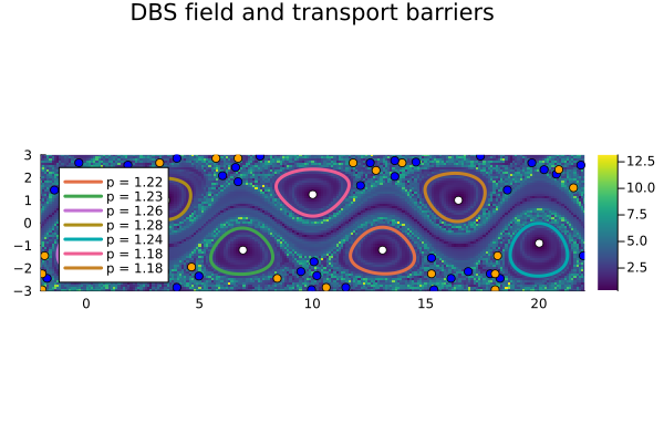
For comparison, we also compute black-hole vortices.
CG_tensor = u -> CG_tensor(bickley, u, tspan, δ; tolerance=1e-6, solver=Tsit5())
C = pmap(CG_tensor, P; batch_size=ceil(Int, length(P)/nprocs()^2))
p = LCSParameters(2.0)
BHvortices, singularities = ellipticLCS(C, xspan, yspan, p)
Finally, we plot them on top of the material diffusion barriers in thin red lines.
foreach(v -> plot_barrier!(v.barriers[1]; color=:red, width=1), BHvortices)
fig
Geostrophic ocean surface flow
Here, we demonstrate how to detect material barriers to diffusive transport.
using Distributed
nprocs() == 1 && addprocs()

@everywhere using CoherentStructures, OrdinaryDiffEq
Next, we load and interpolate the velocity data sets. Loading the data sets defines Lon, Lat, Time, UT, VT.
using JLD2
lon, lat, time, us, vs = load("docs/examples/Ocean_geostrophic_velocity.jld2", "Lon", "Lat", "Time", "UT", "VT")
const VI = interpolateVF(lon, lat, time, us, vs)
Since we want to use parallel computing, we set up the integration LCSParameters on all workers, i.e., @everywhere.
q = 91
t_initial = minimum(time)
t_final = t_initial + 90
const ts = range(t_initial, stop=t_final, length=q)
xmin, xmax, ymin, ymax = -4.0, 7.5, -37.0, -28.0
nx = 300
ny = floor(Int, (ymax - ymin) / (xmax - xmin) * nx)
xspan = range(xmin, stop=xmax, length=nx)
yspan = range(ymin, stop=ymax, length=ny)
P = tuple.(xspan, permutedims(yspan))
const ε = 1.e-5
mcg_tensor = u -> av_weighted_CG_tensor(interp_rhs, u, ts, ε;
    p=VI, tolerance=1e-6, solver=Tsit5())
Now, compute the averaged weighted Cauchy-Green tensor field and extract elliptic LCSs.
C̅ = pmap(mcg_tensor, P; batch_size=ceil(Int, length(P)/nprocs()^2))
p = LCSParameters(2.5)
vortices, singularities = ellipticLCS(C̅, xspan, yspan, p)
Finally, the result is visualized as follows.
using Plots
trace = tensor_invariants(C̅)[5]
fig = plot_vortices(vortices, singularities, (xmin, ymin), (xmax, ymax);
    bg=trace, xspan=xspan, yspan=yspan, title="DBS field and transport barriers", showlabel=true)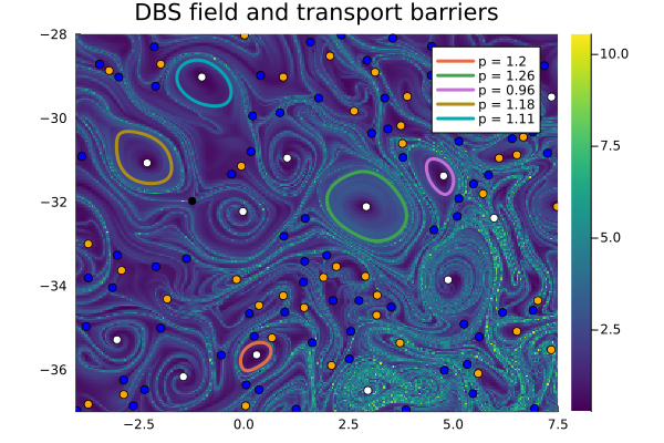
This page was generated using Literate.jl.